\[ \begin{align}\begin{aligned}\newcommand\blank{~\underline{\hspace{1.2cm}}~}\\% Bold symbols (vectors)
\newcommand\bs[1]{\mathbf{#1}}\\% Poor man's siunitx
\newcommand\unit[1]{\mathrm{#1}}
\newcommand\num[1]{#1}
\newcommand\qty[2]{#1~\unit{#2}}\\\newcommand\per{/}
\newcommand\squared{{}^2}
%
% Scale
\newcommand\milli{\unit{m}}
\newcommand\centi{\unit{c}}
\newcommand\kilo{\unit{k}}
\newcommand\mega{\unit{M}}
%
% Angle
\newcommand\radian{\unit{rad}}
\newcommand\degree{\unit{{}^\circ}}
%
% Time
\newcommand\second{\unit{s}}
%
% Distance
\newcommand\meter{\unit{m}}
\newcommand\m{\meter}
\newcommand\inch{\unit{in}}
\newcommand\feet{\unit{ft}}
\newcommand\mile{\unit{mi}}
\newcommand\mi{\mile}
%
% Volume
\newcommand\gallon{\unit{gal}}
%
% Mass
\newcommand\gram{\unit{g}}
\newcommand\g{\gram}
%
% Frequency
\newcommand\hertz{\unit{Hz}}
\newcommand\rpm{\unit{rpm}}
%
% Voltage
\newcommand\volt{\unit{V}}
\newcommand\V{\volt}
\newcommand\millivolt{\milli\volt}
\newcommand\mV{\milli\volt}
\newcommand\kilovolt{\kilo\volt}
\newcommand\kV{\kilo\volt}
%
% Current
\newcommand\ampere{\unit{A}}
\newcommand\A{\ampere}
\newcommand\milliampereA{\milli\ampere}
\newcommand\mA{\milli\ampere}
\newcommand\kiloampereA{\kilo\ampere}
\newcommand\kA{\kilo\ampere}
%
% Resistance
\newcommand\ohm{\Omega}
\newcommand\milliohm{\milli\ohm}
\newcommand\kiloohm{\kilo\ohm} % correct SI spelling
\newcommand\kilohm{\kilo\ohm} % "American" spelling used in siunitx
\newcommand\megaohm{\mega\ohm} % correct SI spelling
\newcommand\megohm{\mega\ohm} % "American" spelling used in siunitx
%
% Inductance
\newcommand\henry{\unit{H}}
\newcommand\H{\henry}
\newcommand\millihenry{\milli\henry}
\newcommand\mH{\milli\henry}
%
% Temperature
\newcommand\celsius{\unit{^{\circ}C}}
\newcommand\C{\unit{\celsius}}
\newcommand\fahrenheit{\unit{^{\circ}F}}
\newcommand\F{\unit{\fahrenheit}}
\newcommand\kelvin{\unit{\K}}
\newcommand\K{\unit{\kelvin}}\\% Power
\newcommand\watt{\unit{W}}
\newcommand\W{\watt}
\newcommand\milliwatt{\milli\watt}
\newcommand\mW{\milli\watt}
\newcommand\kilowatt{\kilo\watt}
\newcommand\kW{\kilo\watt}
%
% Torque
\newcommand\ozin{\unit{oz}\text{-}\unit{in}}
\newcommand\newtonmeter{\unit{N\text{-}m}}\end{aligned}\end{align} \]
Apr 16, 2025 | 120 words | 1 min read
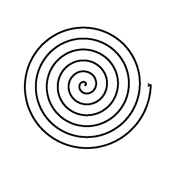
6.2.4. SpiralStarting with the code provided in spiral_login.py main
(6.1) \[x = \frac{\theta_\text{degrees}}{\pi^2} \cos(\theta_\text{radians})\]
(6.2) \[y = \frac{\theta_\text{degrees}}{\pi^2} \sin(\theta_\text{radians})\]
where \(\theta_\text{degrees}\) increases from \(0^{\circ}\) .
Note
Note that in these equations, \(\theta_{degrees}\) is in degrees, but that
the sin and cos functions in Python expect their argument to be in
radians. You can convert from degrees to radians using
(6.3) \[\theta_\text{radians} = \frac{\pi}{180^{\circ}} \theta_\text{degrees}\]
or by using the radians math
Sample Output
Compare your program’s output to the provided sample output.
Fig. 6.2 Case_1_spiral.png
Deliverables
Save your finished program as spiral_login.py login Table 6.6